
Meaning and mechanism
If the number of predators increases, the predators may obtain a larger food supply. If predator increases lead to a decrease in the prey population, then the changes in both groups are linked.
It takes time for an increase in the food supply to lead to an increase in the predator’s population. Therefore, we can explain the tendency for the peak of the predator to appear after the peak of the prey.
Relationships and conditions
The Lotka-Volterra model combines an increase in the predator, αx, with a predation rate, βxy, and an increase in the predator, δxy, and a decrease, γy. The predation terms are related to the frequency with which the two populations encounter each other.
Classical models omit the prey’s resource limitation, the predator’s satiation, and refuge. Actual ecosystems do not always draw constant closed cycles.
What to observe in the simulation
As prey increases, predators follow suit, and as predation pressure increases, prey decreases. Outside of equilibrium, it moves in a closed orbit.
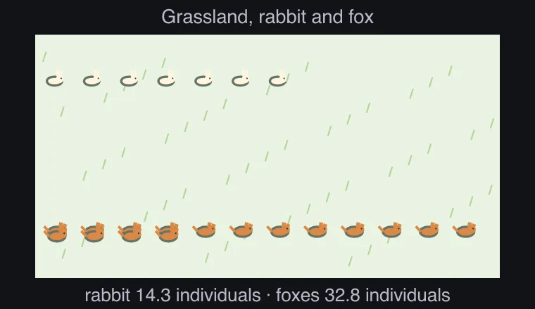
It is a Lotka-Volterra model with a closed population without immigration or exodus, unlimited food resources, uniform encounters, and constant coefficients. RK4 spacing is 1/60 model time. We omit the environmental carrying capacity, diseases, seasons, shelter, and contingencies of the actual ecosystem. One icon is approximately 2 items, and a maximum of 90 can be drawn. The time difference is averaged only for the completed maximum value pairs, and if there are no pairs in the interval, it is displayed as unmeasured.
Key relationships and symbols
dx/dt=αx−βxy · dy/dt=δxy−γy
| Symbol | Meaning | Unit |
|---|---|---|
| x, y | Prey and predator population sizes | individuals |
| α, β, δ, γ | Model coefficients for growth, predation, and decline | Units depend on the equation |
Worked example
What is the equilibrium point at which the two populations remain unchanged?
dx/dt=x(α−βy), dy/dt=y(δx−γ). The positive equilibrium where both are 0 is x*=γ/δ, y*=α/β.
Common misconceptions
- The number of predators and prey is not always simultaneously increasing or simultaneously decreasing.